Image Processing using Singular Value Decomposition
Suppose a satellite takes a picture and wants to send it to earth. The picture may contain 1000 by 1000 “pixels” – little squares each with a definite color. We can code the colors, in a range between black and white, and send back 1,000,000 numbers. It is better to find the essential information in the 1000 by 1000 matrix, and send only that.
Suppose we know the SVD. The key is in the singular values (in ∑). Typically, some are significant and others are extremely small. If we keep 60 and throw away 940, then we send only the corresponding 60 columns of Q1 and Q2.
…
If only 60 terms are kept, we send 60 times 2000 numbers instead of a million.
The pictures are really striking, as more and more singular values are included. At first you see nothing, and suddenly you recognize everything.
Gilbert Strang, Linear Algebra And Its Applications 3:d edition, Appendix A
I distincly remember reading this as a student many years ago, imagining what the results would be, but never actually tried it – until now.
The basic idea is very simple. A digital image, with its pixels, is essentially a matrix. Each element of the matrix is a number representing the colour of the corresponding pixel. (To keep things simple we’ll limit this example to monochrome/greyscale images.) All matrices have a Singular Values Decomposition (SVD), and the original matrix can be reconstructed from the SVD. When we perform that reconstruction we can choose to disregard some components. In particular, with the SVD, components corresponding to (relatively) small singular values can be left out. If the components left out are not too many and they correspond to small singular values, you won’t notice a difference in the reconstructed matrix/image. Components that are not used in the reconstruction can be completely discarded – no need to store or transmit them.
The code example below demonstrates how to do this with ojAlgo. The images in the animation above were generated using that program. You can try it with any image you have available (any file formats supported by java.awt.image.BufferedImage).
In the animation there are 9 reconstructed images displayed in order of increasing “rank” with 1s delay in between each. At the end the full/original image is displayed for 6s. (The animation takes 15s in total.) The table below shows with what rank the images were recreated, as well as how many bytes need to be stored in that case paired with how many bytes where discarded (saved).
| # | Rank | Store (bytes) | Discard (bytes) | Saving |
|---|---|---|---|---|
| 1 | 1 | 1,999 | 919,601 | 99,78 % |
| 2 | 2 | 3,996 | 917,604 | 99,57 % |
| 3 | 5 | 9,975 | 911,625 | 98,92 % |
| 4 | 10 | 19,900 | 901,700 | 97,84 % |
| 5 | 20 | 39,600 | 882,000 | 95,70 % |
| 6 | 50 | 97,500 | 824,100 | 89,42 % |
| 7 | 100 | 19,0000 | 731,600 | 79,38 % |
| 8 | 200 | 360,000 | 561,600 | 60,94 % |
| 9 | 500 | 750,000 | 171,600 | 18,62 % |
In that quote from Gilbert Strang it was stated that for a 1000 by 1000 matrix, where we keep only 60 columns in each of Q-matrices we would transmit/store 60x2x1000 pixels/bytes. I believe this can be taken one step further. Due to how an SVD is stored internally, the number of discarded bytes would instead by (940×940). You typically don’t store the columns of the Q-matrices, but the Householder-vectors used to create them, and that means there’s further structure that can be exploited to save “space”. In the table I estimated the savings that way.
If a matrix/image has m rows and n columns, but only r components of the SVD are stored, then:
- The full image is
m*nbytes - An SVD can essentially be calculated/stored in-place (requiring
m*nbytes) - The number of bytes that can be discarded is
(m-r)*(n-r) - Resulting in
(m*n) - ((m-r)*(n-r))bytes to store
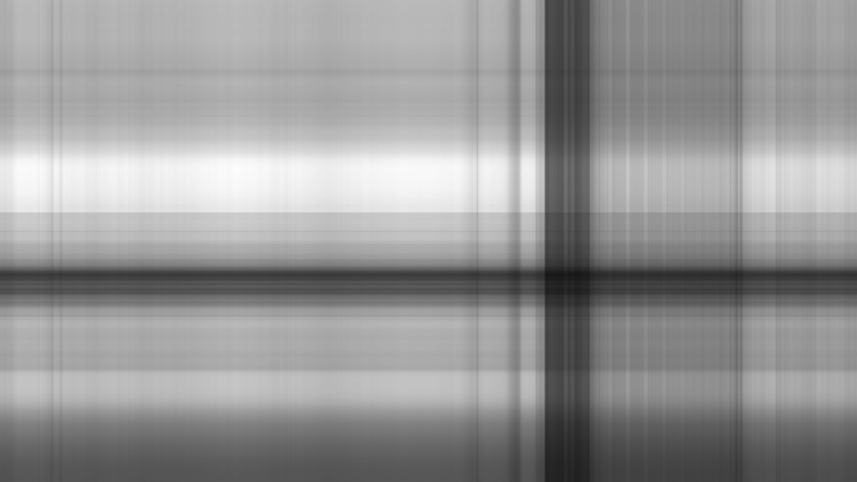
It’s important to remember that even with a rank=1 reconstruction, the recreated matrix/image is full resolution. What we get when we include more components is more information on what colour each of the pixels should be, but we always have the same number of pixels. In the above animation all the images are 1280×720 pixels. The first image is the rank=1 recreation. There’s no way to see what’s in that picture, but as we add more components the picture evolves rapidly. Already with image number 3 (rank=5) we recognise the original, and with rank=10 you could probably tell what the picture is of even if you hadn’t seen the original. At rank=50 all the main shapes are there, with rank=100 most details as well, but still with some distortions/smearing in the image. At rank=200 the image is virtually indistinguishable from the original, and that’s with 61% storage saving.
Removing a few of the smallest singular values could even be interpreted as improving the image, as it removes noise in the image representation.
ImageProcessingSVD.javaimport java.io.File;
import java.io.IOException;
import org.ojalgo.OjAlgoUtils;
import org.ojalgo.array.Array1D;
import org.ojalgo.data.image.ImageData;
import org.ojalgo.function.aggregator.Aggregator;
import org.ojalgo.matrix.decomposition.SingularValue;
import org.ojalgo.matrix.store.MatrixStore;
import org.ojalgo.netio.BasicLogger;
import org.ojalgo.netio.ShardedFile;
/**
* Basic image processing using ojAlgo.
* <p>
* Demonstrates how to "compress" an image by removing non-essential information from the image.
*
* @see https://www.ojalgo.org/2023/10/image-processing-using-singular-value-decomposition/
*/
public class ImageProcessingSVD {
private static final File BASE_DIR = new File("/Users/apete/Developer/data/compression/");
public static void main(final String[] args) throws IOException {
BasicLogger.debug();
BasicLogger.debug(ImageProcessingSVD.class);
BasicLogger.debug(OjAlgoUtils.getTitle());
BasicLogger.debug(OjAlgoUtils.getDate());
BasicLogger.debug();
File inputFile = new File(BASE_DIR, "cityhall.png");
/*
* Read any image file (supported by java.awt.image.BufferedImage) and convert it to a grey scale
* image.
*/
ImageData initialImage = ImageData.read(inputFile).convertToGreyScale();
/*
* The length of the diagonal is also the number of singular values
*/
int nbDiagonal = initialImage.getMinDim();
int nbRows = initialImage.getRowDim();
int nbCols = initialImage.getColDim();
/*
* 1 byte per pixel in the image.
*/
double storageRequirement = nbRows * nbCols;
/*
* Never mind "sharded". This is just a convenient way to keep track of multiple files with unique
* numbers as part of the file names.
*/
ShardedFile outputFiles = ShardedFile.of(BASE_DIR, "resampled.png", 1 + nbDiagonal);
/*
* Write the original, grey scale, image to disk.
*/
File originalGreyScaleFile = outputFiles.single;
initialImage.writeTo(originalGreyScaleFile);
/*
* Calculate the SVD
*/
SingularValue<Double> decomposition = SingularValue.R064.decompose(initialImage);
Array1D<Double> singularValues = decomposition.getSingularValues();
double largestSingularValue = singularValues.doubleValue(0);
double sumOfAllSingularValues = singularValues.aggregateAll(Aggregator.SUM);
double conditionNumber = decomposition.getCondition();
BasicLogger.debug("Largest singular value={}, Sum of all={}, Condition number={}", largestSingularValue, sumOfAllSingularValues, conditionNumber);
BasicLogger.debug();
BasicLogger.debug("Rank SingularValue Rel.Mag. Aggr.Info Storage");
BasicLogger.debug("=================================================");
int[] ranks = { 1, 2, 5, 10, 20, 50, 100, 200, 500, 1000, 2000, 5000 };
for (int r = 0, rank = 0; r < ranks.length && (rank = ranks[r]) <= nbDiagonal; r++) {
/*
* Here rank refers to the number of singular values (the number of components) used when
* reconstructing the matrix.
*/
/*
* If the rank is N then this is the N:th largest singular value (zero-based index)
*/
double singularValue = singularValues.doubleValue(rank - 1);
/*
* and this is the sum of the N first/largest singular values.
*/
double sumOfSingularValues = singularValues.aggregateRange(0, rank, Aggregator.SUM);
/*
* The part of the SVD storage we don't need when reconstructing the matrix at this rank.
*/
double noNeedToStore = (nbRows - rank) * (nbCols - rank);
BasicLogger.debugFormatted("%4d %14.2f %9.4f %9.2f%% %7.2f%%", rank, singularValue, singularValue / largestSingularValue,
100.0 * sumOfSingularValues / sumOfAllSingularValues, 100.0 * (storageRequirement - noNeedToStore) / storageRequirement);
/*
* Reconstruct the matrix using 'rank' number of components.
*/
MatrixStore<Double> recreatedMatrix = decomposition.reconstruct(rank);
/*
* Copy that matrix to a new image
*/
ImageData recreatedImage = ImageData.copy(recreatedMatrix);
/*
* Write that image to file (with the rank as part of the file name)
*/
File outputFile = outputFiles.shard(rank);
recreatedImage.writeTo(outputFile);
}
}
}
Console Output
Running the above program gives the following output.
class ImageProcessingSVD
ojAlgo
2023-10-16

Largest singular value=193027.35715261783, Sum of all=353664.140238967, Condition number=43424.72711999176

Rank  SingularValue  Rel.Mag.  Aggr.Info  Storage
=================================================
   1      193027.36    1.0000     54.58%    0.22%
   2       12799.36    0.0663     58.20%    0.43%
   5        6995.57    0.0362     65.12%    1.08%
  10        2810.83    0.0146     70.10%    2.16%
  20        1458.08    0.0076     75.65%    4.30%
  50         665.87    0.0034     83.66%   10.58%
 100         314.76    0.0016     90.12%   20.62%
 200         117.42    0.0006     95.66%   39.06%
 500          15.24    0.0001     99.41%   81.38%
- ← Previous
ojAlgo v53.1.0 - Next →
Image Processing using FFT